Cahill-Keyes geometric context
Documentation index · Implementation notes · Bibliography
What kind of projection this is
The Cahill-Keyes is a polyhedral world map. Conceptually, the globe is divided among the eight triangular faces of an octahedron: four faces meet at the North Pole and four at the South Pole. Each spherical face covers 90 degrees of longitude and one hemisphere. Unfolding and arranging those faces produces the characteristic Cahill-Keyes M-shaped map.
This construction is unlike a cylindrical projection with one formula applied continuously across a rectangular longitude-latitude grid. It deliberately has cuts between selected octants. Within an octant, meridians and parallels are constructed piecewise to control the relative shape and scale of geographic cells. The implementation therefore follows a geometric construction rather than a single closed-form equation.
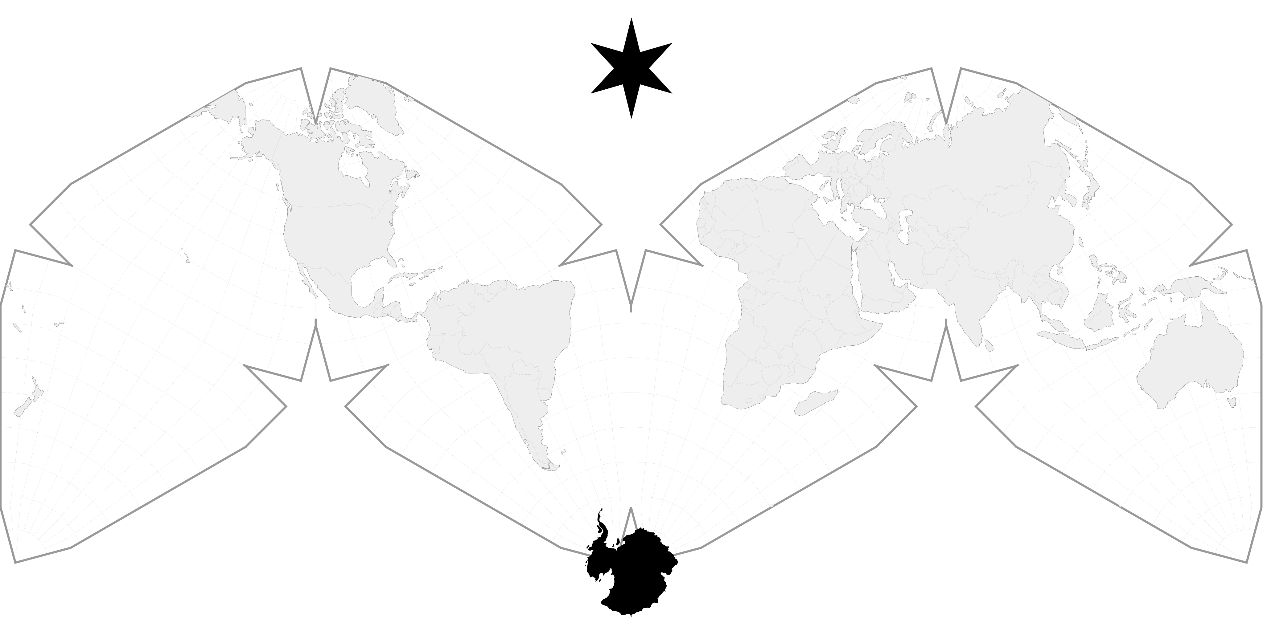
The illustration is the checked-in 44-by-22-inch Visionscarto SVG. Its outer frame has the required 2:1 ratio. The graticule exposes the triangular octants, the repeated polar vertices, and the intentional gaps at the map’s cuts.
Quadrants, octants, and half-octants
“Quadrant” is useful as a general orientation term, but the construction’s algorithmic unit is an octant. A hemisphere has four 90-degree longitude sectors; adding north and south makes eight spherical octants. The seams are rotated relative to the prime meridian, so the ordinary northeast, northwest, southeast, and southwest geographic quadrants do not coincide with projection faces.
The canonical numbering inherited from MegamapMaker-prep9.pl is:
| Longitude sector | North | South | Broad geographic context |
|---|---|---|---|
| 160° E through 180° and 180° through 110° W | 1 | 6 | Pacific, western North America, New Zealand |
| 110° W to 20° W | 2 | 7 | North America and North Atlantic; South America |
| 20° W to 70° E | 3 | 8 | Europe, Africa, and the Middle East |
| 70° E to 160° E | 4 | 5 | Asia; Australia |
flowchart TB
  NP((North Pole))
  SP((South Pole))

  subgraph N[Four northern octants]
    N1["1<br/>Pacific"]
    N2["2<br/>Americas / Atlantic"]
    N3["3<br/>Europe / Africa"]
    N4["4<br/>Asia"]
  end

  subgraph S[Four southern octants]
    S6["6<br/>Pacific"]
    S7["7<br/>South America"]
    S8["8<br/>South Africa"]
    S5["5<br/>Australia"]
  end

  NP --- N1
  NP --- N2
  NP --- N3
  NP --- N4
  N1 --- S6
  N2 --- S7
  N3 --- S8
  N4 --- S5
  S6 --- SP
  S7 --- SP
  S8 --- SP
  S5 --- SP
This diagram shows geographic pairing, not the final planar positions. The rotations and translations that form the M-layout are described below.
Each octant is itself split down its central meridian. All coordinate construction can then happen in one reference half-octant:
p = |latitude|is the parallel, from 0° at the equator to 90° at a pole.mis the absolute angular distance from the octant’s central meridian, from 0° on the center line to 45° on an outer edge.- A sign records which side of the center line supplied the point. It mirrors the reference coordinate before octant assembly.
Thus eight octants become sixteen mirrored half-octants, but the difficult geometry is calculated only once.
Geometry inside the reference half-octant
The template starts with the 10,000-unit scaffold MG. Important points on
the center line, equator, outer boundary, and transition curves establish the
graticule. Rays and line intersections form each meridian’s torrid, middle,
and frigid segments. Circular arcs control the polar region. A specially
constructed circle supplies the 15° transition through the “supple” zones near
the outer third of the octant.
The original construction names twelve regions A through L. Dispatch order matters where their boundary conditions overlap:
flowchart TD
  IN["Reference coordinate<br/>0° ≤ m ≤ 45°, 0° ≤ p ≤ 90°"] --> M0{"m = 0°?"}
  M0 -- yes --> AB["A / B<br/>octant center line"]
  M0 -- no --> P75{"p ≥ 75°?"}
  P75 -- yes --> C["C<br/>polar circular arc"]
  P75 -- no --> P0{"p = 0°?"}
  P0 -- yes --> D["D<br/>equator"]
  P0 -- no --> ETEST{"p ≥ 73° and m ≤ 30°?"}
  ETEST -- yes --> E["E<br/>polar transition"]
  ETEST -- no --> M45{"m = 45°?"}
  M45 -- yes --> FGH["F / G / H<br/>outer boundary"]
  M45 -- no --> M29{"m ≤ 29°?"}
  M29 -- yes --> I["I<br/>central two-thirds"]
  M29 -- no --> JTEST{"p ≥ 73°?"}
  JTEST -- yes --> J["J<br/>frigid supple zone"]
  JTEST -- no --> P15{"p ≤ 15°?"}
  P15 -- yes --> K["K<br/>torrid supple zone"]
  P15 -- no --> L["L<br/>middle supple zone"]
The purpose of the piecewise construction is continuity through the intended joins while preserving Keyes’s chosen proportions. A point may be computed by linear interpolation along a constructed meridian, by a polar circular arc, or by a line-circle intersection, depending on its zone. The exact formulas are in the implementation notes.
From one template to the M-layout
After constructing (x, y) in the reference half-octant, the longitude-side
sign mirrors y. The result is rotated and translated according to its octant.
Southern octants first reflect the template horizontally about x = MG.
| Octant | Southern reflection | Rotation | Horizontal translation |
|---|---|---|---|
| 1 | no | -120° | -MG |
| 2 | no | -60° | -MG |
| 3 | no | -120° | +MG |
| 4 | no | -60° | +MG |
| 5 | yes | -60° | +MG |
| 6 | yes | -120° | -MG |
| 7 | yes | -60° | -MG |
| 8 | yes | -120° | +MG |
Every octant then receives the same vertical translation,
MG sin(60°). These rigid transformations form the standard M-profile without
changing any local half-octant geometry.
flowchart LR
  LL["latitude, longitude"] --> OCT["choose octant<br/>and half-side"]
  OCT --> MP["normalize to<br/>(m, p, sign)"]
  MP --> XY["A–L reference<br/>construction"]
  XY --> MIRROR["mirror half and<br/>southern octants"]
  MIRROR --> ASSEMBLE["rotate + translate<br/>into M-layout"]
  ASSEMBLE --> FRAME["center and invert y<br/>in a 2:1 frame"]
The 2:1 rendering frame
The canonical scaffold has MG = 10,000 and an M-layout span of 40,000 units.
For a frame of width W and height H, this implementation requires
W = 2H and chooses:
MG = H / 2 = W / 4
frame center = (W / 2, H / 2)
The native construction uses Cartesian coordinates with positive y upward.
Rendering uses screen coordinates with positive y downward, so the final
conversion is:
X = W / 2 + x
Y = H / 2 - y
Scaling only changes lengths, not angles, zone boundaries, octant selection, or relative positions. The same code therefore fits a 44-by-22 logical frame, the 4224-by-2112 SVG coordinate space, the 13200-by-6600 300-DPI raster, and arbitrary fractional 2:1 frames.
Cuts, seams, and paths
A polyhedral projection is discontinuous at its cut edges. The point API makes
a deterministic octant choice at every longitude boundary, but a line or
polygon crossing a cut must be split instead of connected through the blank
space between octants. Projection-specific path handling remains in
cart0freak0-cahill-keyes-functions.h.
The helper views the placed projection as the rectangle bounded by L, R,
T, and B. A large jump between opposite outer quarters or opposite
vertical halves is interpreted as a short wrapped continuation. It terminates
the current path at one edge and begins a new path at the paired edge:
| Projected movement | Current segment exits | Next segment enters |
|---|---|---|
| left outer quarter → right outer quarter | L |
R |
| right outer quarter → left outer quarter | R |
L |
| north half → south half | T |
B |
| south half → north half | B |
T |
The edge point is not copied from either endpoint. It is the intersection of the selected unwrapped line with the frame edge, so a diagonal path remains directionally continuous. A link that crosses both horizontal and vertical edges is split in intersection order; a link aimed exactly through a corner exits and re-enters through the opposite corner.
flowchart LR
  PAIR["adjacent projected points"] --> CLASSIFY["classify opposite<br/>quarters / halves"]
  CLASSIFY --> UNWRAP["shift endpoint by<br/>frame width / height"]
  UNWRAP --> INTERSECT["intersect selected line<br/>with frame edge"]
  INTERSECT --> SPLIT["close at exit<br/>restart at paired entry"]
This is projected-path repair, not spherical clipping. It assumes ordered, reasonably sampled points already produced by the same placed Cahill-Keyes cartography. It deliberately leaves a large jump unchanged when the endpoints do not identify a supported opposite-frame-edge transition. See the implementation notes for the API contract, thresholds, formulas, and example.
The native class provides the authoritative forward construction and an
octant-qualified reverse. The reverse first undoes a selected M-layout
octant and then solves the bounded piecewise half-octant by forward residual.
It does not pretend the interrupted carrier has one globally unique inverse:
the runtime returns explicit candidates and unique, ambiguous, cut, or
outside status. See the
forward/reverse API and the
implementation plan and issues.