Star-X geometric context
Documentation index · Implementation notes · Bibliography
What Star-X changes
Star-X is a rearranged Cahill-Keyes octahedral net. It does not replace the curves inside an octant. The globe is still divided into eight spherical triangles, every triangle still uses the Cahill-Keyes A–L construction, and the same continental cuts remain available. Star-X changes where two groups of those projected faces are placed on the page.
The current specification also defines one composed southern component. The
ordinary X carrier is cut at the geographic parallel 60°S; everything at or
south of that parallel can be reassembled around one bottom-center South Pole.
That boundary, radial transform, zero-degree bearing, and page registration are
projection geometry. They do not depend on a coastline, land extent, or
Natural Earth. Source datasets supply content to clip and draw, not parameters
for the Star-X transform.
The ordinary Cahill-Keyes M map is horizontal. Star-X reads its four north/south face pairs from left to right, keeps the first two pairs in the lower half, rotates the last two pairs by 180 degrees, and puts them in the upper half. The result is a portrait, polar-centered X.
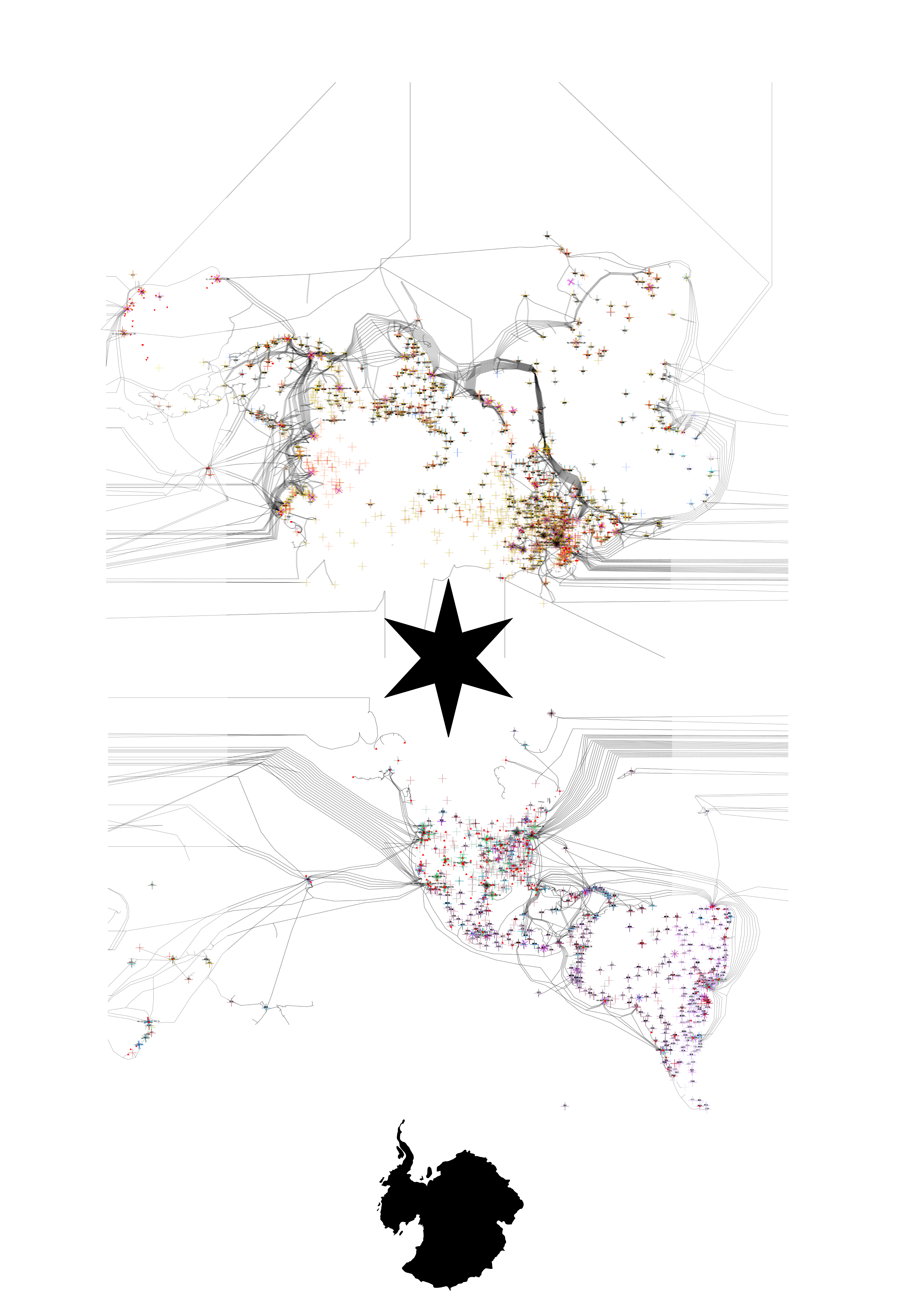
The checked-in image is a historical data visualization and a visual record of the arrangement, not a pixel oracle for the C++ projection. It includes symbols, links, crops, and page-layout decisions beyond the geographic transform.
Octahedral context
An octahedron has eight triangular faces. Four touch its northern vertex and four touch its southern vertex. On the globe these become four 90-degree longitude sectors per hemisphere. Flattening the faces requires cuts; a pole or edge can therefore have several visible copies in a planar net even though it is one location on the folded polyhedron.
The Cahill-Keyes algorithm calculates one mirrored half-octant and then uses rigid rotations, reflections, and translations to form all eight faces. That standard assembly produces the M profile shown in the Cahill-Keyes context. Star-X starts after this calculation, so the local scale and carefully constructed graticule remain unchanged.
Face numbers and spatial slots
Two numbering systems must be kept distinct.
The official geographic octant numbering inherited from the Graça/Keyes program is:
| Longitude sector | North octant | South octant |
|---|---|---|
| Pacific and western North America | 1 | 6 |
| Americas and Atlantic | 2 | 7 |
| Europe, Africa, and Middle East | 3 | 8 |
| Asia and Australia | 4 | 5 |
In the rendered M layout, north and south partners are adjacent. Numbering the triangular spatial slots from left to right therefore gives:
| Spatial slots | Official octants | Source half | Star-X group |
|---|---|---|---|
| 1–2 | 1 and 6 | left, outer | group 1 |
| 3–4 | 2 and 7 | left, inner | group 1 |
| 5–6 | 3 and 8 | right, inner | group 2 |
| 7–8 | 4 and 5 | right, outer | group 2 |
Thus the requested “octants 1–4 on the left” and “octants 5–8 on the right” are spatial slots in the M map. Treating them as official geographic octant numbers would instead split north from south, contradicting the left/right geometry and the historical plate arrangement.
flowchart LR
  subgraph M[Standard Cahill-Keyes M layout]
    Q1["slots 1–2<br/>octants 1 / 6"]
    Q2["slots 3–4<br/>octants 2 / 7"]
    Q3["slots 5–6<br/>octants 3 / 8"]
    Q4["slots 7–8<br/>octants 4 / 5"]
    Q1 --- Q2 --- Q3 --- Q4
  end
From M to X
Split the M-layout rectangle vertically between the second and third face pairs. Each half is square. Group 1 stays upright and moves below the carrier midpoint. Group 2 rotates around the center of its square and moves above the midpoint.
flowchart TB
  SRC["22 × 11 Cahill-Keyes source<br/>[ Q1 ][ Q2 ] | [ Q3 ][ Q4 ]"]
  SPLIT{"split into<br/>11 × 11 groups"}
  G1["group 1<br/>Q1 then Q2<br/>keep orientation"]
  G2["group 2<br/>Q3 then Q4<br/>rotate 180°"]
  PLACE["close the group gap"]
  SCALE["enlarge complete X 120%<br/>about page center"]
  FINAL["17 × 22 Star-X carrier<br/>top: Q4 Q3<br/>center: North-pole star<br/>bottom: Q1 Q2 + Antarctica"]

  SRC --> SPLIT
  SPLIT --> G1 --> PLACE
  SPLIT --> G2 --> PLACE
  PLACE --> SCALE --> FINAL
A compact page diagram is:
17 units wide
┌─────────────────┐
│   ┌─────┬─────┐ │
│   │ Q4↻ │ Q3↻ │ │  group 2, rotated 180 degrees
│   └──╲──┴──╱──┘ │
│        NP         │  northern polar copies bound the X center
│   ┌──╱──┬──╲──┐ │
│   │ Q1  │ Q2  │ │  group 1, original orientation
│   └─────┴─────┘ │
└─────────────────┘
22 units high
Here Q1 through Q4 are the four ordinary Cahill-Keyes north/south face
pairs. A 180-degree rotation reverses both order and orientation, so the
upper row reads Q4, Q3 from left to right. That is the same 4 3 / 1 2
plate ordering documented for the historical composition.
Why the center is the North Pole
In the lower group, northern polar vertices lie along its upper inward boundary. In the rotated upper group they lie along its lower inward boundary. Stacking those boundaries around the carrier midpoint makes the North Pole the conceptual center of the composition.
Because an unfolded polyhedron has cuts, the geographic North Pole is not forced into one shared planar coordinate. Its octant copies form a compact locus around the midpoint. The converging face edges outline an eight-rayed star or X; historical maps place a black star over this area. Preserving the copies maintains continuity inside every octant and avoids an artificial snap at exactly 90 degrees latitude.
The South Pole does not occupy the center. Group 2 carries its southern vertices toward the top edge after rotation, while group 1 carries them toward the bottom edge. The map can therefore be turned 180 degrees without giving one half a permanent visual “top.” Stages 6 and 13 introduced a single South-polar cap at the lower end; Stage 14 fixed its data-independent page registration. It is an explicit layer-aware cut and reassembly, not a collapse of the point projection’s polar copies.
Polar marks and Antarctica
The finished presentation uses two different kinds of polar context. The
North Pole is a symbolic eight-point star over the central locus. Antarctica
is a geographic component of the projection. The final compositor cuts every
source at the fixed 60°S parallel and reassembles all content at or south of
it around one South Pole at bottom center. The same result is obtained for the
same frame and star_x_layout even when no physical-feature dataset is
installed.
This distinction is perceptual as well as numerical. The star makes the rotation center immediately legible without pretending that all cut copies of the North Pole are one topological vertex. The Antarctic cap restores a recognizable continent where the ordinary octahedral net would divide it among outer faces. Every point keeps its original distance from its quadrant tip, so no independent inset scale is introduced. Geographic bearing is normalized around the shared pole to join Cahill-Keyes’s bent octant edges. Ocean, land, bathymetry, ice, linework, and graticules all use the same cap; the southern source portions are removed, so nothing is duplicated. Within each thematic layer, transformed Antarctic paths are serialized after every ordinary quadrant path and therefore paint on top.
The cap registration is fixed by its projected 60°S boundary. Let
L(phi,lambda) be the radius-preserving cap point relative to the shared pole,
in the usual page axes where y increases downward. The pole is registered as:
Cx = W / 2
clearance = H * (0.25 / 44)
Cy = H - clearance - max_lambda(Ly(-60°, lambda))
The boundary is sampled at quarter-degree longitude intervals, including both
antimeridian limits. Therefore its bottommost point is exactly one quarter
unit above the lower edge of a 34 × 44 carrier, with proportional clearance
at every other valid 17:22 size. This is why the blue unified-cap edge remains
visible instead of being clipped by the SVG view box. The placement is a
carrier invariant, not a measurement of the Antarctic mainland.
Quadrants in the final carrier
The portrait carrier has four practical drawing quadrants. They are page regions rather than spherical quadrants:
| Final page quadrant | Source pair | Geographic octants | Orientation |
|---|---|---|---|
| upper left | Q4 | 4 and 5 | rotated 180 degrees |
| upper right | Q3 | 3 and 8 | rotated 180 degrees |
| lower left | Q1 | 1 and 6 | original |
| lower right | Q2 | 2 and 7 | original |
This ordering makes Asia/Australia and Europe/Africa approach the central pole from above, while the Pacific and Americas approach it from below. The equatorial edges and outer octant boundaries create the diagonal strokes that give the net its X silhouette.
Aspect and margins
A tight stack of two square groups would have a 1:2 ratio. Star-X retains the historic four-panel carrier instead: two 17-by-22 portrait panels across and two down make 34 by 44, whose reduced ratio is 17:22.
Using height units, the exact layout is:
frame: 17/22 wide by 1 high
each group: 1/2 wide by 1/2 high
left and right margin: 3/22 each
signed carrier gap: R in [-1/2, 0]
default R: -9/88
page-centered enlargement E > 0
default E: 6/5
The margins are part of the frame contract, not anisotropic padding added
after projection. Both group squares, their vertical spacing, and every
Cahill-Keyes construction length scale uniformly with frame.height().
The “carrier gap” is signed because it describes the spacing between the
two invisible square source regions. R=0 gives their former edge-to-edge
placement. A negative value overlaps those regions while leaving every
octant rigid. The default R=-9/88 translates each group inward by
9/176 of frame height. On the 34-by-44 generated example that is exactly
2.25 units per group: the lower group rises and the upper group descends
toward the 22-unit centerline. Passing a zero ratio remains available when
the older, wider central opening is desired.
After the gap is closed, the complete arrangement is uniformly enlarged
about the page center. The default 6/5 factor reduces the historical margins
without changing the 17:22 page ratio or distorting any face. On the
34-by-44 page this is the affine translation-and-scale
matrix(1.2,0,0,1.2,-3.4,-4.4).
Cuts and continuity
Within one half-octant the projection is continuous. Discontinuities occur at selected octant edges, at the standard M-layout wrap, and at the new left/right group split. Those cuts are the price of laying an octahedral surface flat.
A renderer should group or clip a coastline, graticule, or network path by
face before drawing. If two adjacent geographic samples project to opposite
parts of the page, joining them directly can draw a false line across the
carrier. Point markers such as those in augment_carto_geo_specific need no
special seam treatment.
Orientation summary
flowchart TD
  LL["latitude / longitude"]
  CK["Cahill-Keyes half-octant formula"]
  M["assemble ordinary M-layout point"]
  SIDE{"native x < 0?"}
  LOWER["group 1<br/>translate to lower square"]
  UPPER["group 2<br/>rotate 180° and translate to upper square"]
  GAP["apply symmetric<br/>signed group gap"]
  ENLARGE["uniformly enlarge about<br/>the page center"]
  FRAME["scale into<br/>frame.frame_area"]
  COMPOSE["SVG composition:<br/>central star + fixed-60°S unified cap"]

  LL --> CK --> M --> SIDE
  SIDE -- yes --> LOWER --> GAP
  SIDE -- no --> UPPER --> GAP
  GAP --> ENLARGE --> FRAME
  FRAME -. layer-aware generation .-> COMPOSE
The checked API 3 runtime implements both components of the current Star-X
forward and reverse transformation. Carrier component 0 reverses the Star-X
group transform before applying the checked Cahill–Keyes inverse. Unified-cap
component 1 recovers bearing around its registered South Pole and solves the
bounded source-radius equation on [-90°,-60°]. A result retains a component
identifier because the ordinary carrier and the top-painted cap can occupy
overlapping page regions. The forward/reverse API
defines candidate, cutoff, quadrant-seam, overlap, and South-Pole behavior.